Jaynes-Cummings model

Code

import imp
qo = imp.load_module("pyqo", *imp.find_module("pyqo", [".."]))
import numpy as np

N = 10 # dimension of field Hilbert space
delta_c = 1
delta_a = 2
g = 1
gamma = 0.1
kappa = 0.1

# Field
id_f = qo.identity(N)
a = qo.destroy(N)
at = qo.create(N)
n = qo.number(N)

# Atom
id_a = qo.identity(2)

# Initial state
psi_0 = qo.basis(N,0) ^ qo.basis(2,1)

# Hamiltonian
H = delta_c*(at*a^id_a)\
    + delta_a*(id_f^qo.sigmap*qo.sigmam)\
    + g*(a^qo.sigmap) + g*(at^qo.sigmam)

# Solve Master equation
T = np.linspace(0, 2*np.pi, 30)
rho = qo.solve_ode(H, psi_0, T,
        [gamma**(1/2)*(id_f^qo.sigmam), kappa**(1/2)*(a^id_a)])

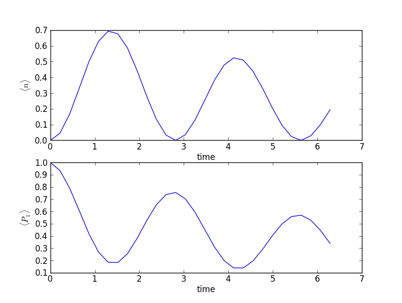
# Expectation values
n_exp = qo.expect(n^id_a, rho)
e_exp = qo.expect(id_f^qo.sigmap*qo.sigmam, rho)

# Q-function
x = np.linspace(-4,4,40)
y = np.linspace(-4,4,40)
X, Y = np.meshgrid(x,y)


# Visualization
import pylab
pylab.figure(1)
pylab.subplot(211)
pylab.xlabel("time")
pylab.ylabel(r"$\langle n \rangle$")
pylab.plot(T, n_exp)
pylab.subplot(212)
pylab.xlabel("time")
pylab.ylabel(r"$\langle P_1 \rangle$")
pylab.plot(T, e_exp)
pylab.show()

Q = []
for rho_t in rho:
    rho_f = qo.ptrace(rho_t,1)
    Q.append(np.abs(qo.qfunc(rho_f,X,Y)))

def qplot(fig,step):
    axes = fig.add_subplot(111)
    axes.clear()
    axes.imshow(Q[step])

qo.animate(len(rho), qplot)

Output